As part of our Computer Graphics course, we were required to implement the infamous “Seam Carving” algorithm. The catch was, we were told to use an approximation of Canny Edge Detection, a difficult exercise in its own right. This approximation was to first blur the image using a 5x5 Gaussian blur, followed by determining the gradient using a 3x3 Sobel operator. From here our problems started.
Caveat: I am a student, I do not claim to understand the topic about which this post is written. Rather I claim not to know (it’s a sort of rant).
First off, none of us had the mathematical background to understand Fourier Transforms, and thus we lacked an in-depth understanding of image convolution. I ended up checking out a book on Digital Image Processing (Gonzalas & Woods, 1992) from the library in an attempt to understand the underlying mathematics better.
Over several attempts, I found that the original formula for a Gaussian function as a 2D plane:

g(x,y,sigma) = (1.0 / (2.0 * pi * sigma * sigma)) * e^(-(x*x+y*y)/(2.0*sigma*sigma))Gave values that made little sense to me, especially given my lack of mathematical understanding. But I needed a way to quickly see the error, so I decided to “normalize” the kernel, based upon it’s minimum value (multiplying all other values in the kernel by the inverse ratio). Thus, I was able to build a kernel with integer values, which is a lot easier to compare by sight with the typical gaussian blur kernel that was given to us:
[ 1,  2,  3,  2, 1 ]
[ 2,  7, 11,  7, 2 ]
[ 3, 11, 17, 11, 3 ]
[ 2,  7, 11,  7, 2 ]
[ 1,  2,  3,  2, 1 ]
The first time I ran it, it didn’t work very well, since apparently my choice of sigma values was still incorrect. I starting searching on Google for any advice as to what sigma to select, and found little solid reference, mostly finding programmatic references on how to use existing kernels, or how to utilize functions that already generate them, but no direction as to how to select an appropriate size based on a sigma, or viceversa. I finally found some reference in an obscure Java API that mentions how a gaussian function falls off to 0 very quickly beyond a radius of e^(-0.5). It makes perfect sense, seeing it now, but I know that I wouldn’t have thought of it on my own, especially with other, and more pressing issues to deal with.
So I decided to try and set the sigma as such:
sigma = radius * Math.exp(-0.5)And it worked. Almost. While the values weren’t perfect, they were close. They even matched a blog post I found. By extension, it meant that my functions were in line with the wikipedia article, and hopefully, by further extension, generally held convention. However, this wasn’t quite enough. So I tried to improve it further.
It bothered me that my values were still of by 1 or two units, especially in the center, and even more so for different radius masks. So I read the book, skimming over irrelevant parts, and most of the math (I’d love to actually sit down and read it, it seemed interesting). It mentioned something very interesting, in that while the gaussian frequency filter has the same shape as a gaussian spatial filter, it is not the same.
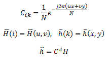
However, later in the same chapter, the book described a method for generating spatial convolution masks from frequency domain filters (such as my Gaussian function). The problem is, this method, while correct, requires an amount of skill as a programmer that I wouldn’t dare to claim (specifically determining the pseudoinverse). Here are the equations:

Where H is the Fourier transform of the frequency filter, ĥ is the spatial filter, N is the size of the frequency sampling, and C# is the pseudoinverse.
While this isn’t such an overly daunting task to program, it is extremely difficult, and there’s not a chance that I would want to do so. So until someone publishes an open source library for doing so, I’ll just have to have blind faith in my TA and his ability to provide the proper assignment materials.
By the way: Mathematica has functions that do this.